


Learn how to scale logistic regression to massive datasets using GPUs and TPUs with PyTorch Lightning Bolts.
This logistic regression implementation is designed to leverage huge compute clusters (Source)
Logistic regression is a simple, but powerful, classification algorithm. In this blog post we’ll see that we can view logistic regression as a type of neural network.
Framing it as a neural network allows us to use libraries like PyTorch and PyTorch Lightning to train on hardware accelerators (like GPUs/TPUs). This enables distributed implementations that scale to massive datasets.
In this blog post I’ll illustrate this link by connecting a NumPy implementation to PyTorch.
I’ve added this highly scalable logistic regression implementation to the PyTorch Lightning Bolts library which you can easily use to train on your own dataset.

All the code examples we’ll walk through can be found in this matching Colab notebook if you’d like to run the code in each step yourself.
Much like other ML libraries (e.g. Sci-kit Learn) this implementation will allow you to fit a logistic regression model in a few lines of code. Unlike other libraries, you’ll be able to train massive datasets on multiple GPUs, TPUs, or CPUs, across many machines.
Beyond toy datasets with a dozen or so features, real datasets may have tens of thousands of features and millions of samples. At this scale, CPUs simply won’t do. Instead, we can leverage GPU and TPUs to turn days of training into minutes.
For example, at the end of this tutorial we train on the full MNIST dataset containing 70,000 images and 784 features on 1 GPU in just a few seconds. And in fact, we have even tried ImageNet. Our logistic regression implementation can loop through all 1.3million images, each with 150,528 pixels (input features) in about 30 minutes on 2 GPUs (V100s).
No matter the complexity of your classification problem, it is always good practice to set a strong baseline using a logistic regression classifier. Even if you intend to use more complex approaches such as neural networks.
The advantage of starting with a logistic regression baseline implemented in PyTorch, is that it makes it easy to swap out the logistic regression model with a neural network.
If you’re familiar with logistic regression feel free to skip this section.
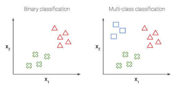
We use logistic regression to predict a discrete class label (such as cat vs. dog), this is also known as classification. This differs from regression where the goal is to predict a continuous real-valued quantity (such as stock price).
In the simplest case of logistic regression, we have just 2 classes, this is called binary classification.
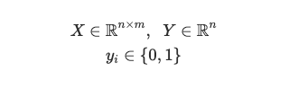
Our goal in logistic regression is to predict a binary target variable Y (i.e. 0 or 1) from a matrix of input values or features, X. For example, say we have a group of pets and we want to find out which is a cat or a dog (Y) based on some features like ear shape, weight, tail length, etc. (X). Let 0 denote cat, and 1 denote dog. We have n samples, or pets, and m features about each pet:
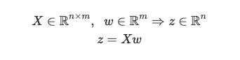
We want to predict the probability that a pet is a dog. To do so, we first take a weighted sum of the input variables — let w denote the weight matrix. The linear combination of the features X and the weights w is given by the vector z.
Next, we apply the sigmoid function to every element of the z vector which gives the vector y_hat.

The sigmoid function, also known as the logistic function, is an S-shaped function that “squashes” the values of z into the range [0,1].
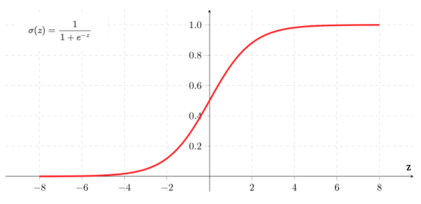
Since each value in y_hat is now between 0 and 1, we interpret this as the probability that the given sample belongs to the “1” class, as opposed to the “0” class. In this case, we’d interpret y_hat as the probability that a pet is a dog.
Our goal is to find the best choice of the w parameter. We want to find a w such that the probability P(y=1|x) is large when x belongs to the “1” class and small when x belongs to the “0” class (in which case P(y=0|x) = 1 — P(y=1|x) is large).
Notice that each model is fully specified by the choice of w. We can use the binary cross entropy loss, or log loss, function to evaluate how well a specific model is performing. We want to understand how “far” our model predictions are from the true values in the training set.
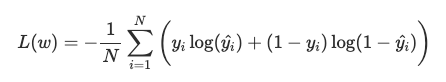
Note that only one of the two terms in the summation is non-zero for each training example (depending on whether the true label y is 0 or 1). In our example, when we have a dog (i.e. y = 1) minimizing the loss means we need to make y_hat = P(y=1|x) large. If we have a cat (i.e. y = 0) we want to make 1 — y_hat = P(y=0|x) large.
Now we have loss function that measures how well a given w fits our training data. We can learn to classify our training data by minimizing L(w) to find the best choice of w.
One way in which we can search for the best w is through an iterative optimization algorithm like gradient descent. In order to use the gradient descent algorithm, we need to be able to calculate the derivative of the loss function with respect to w for any value of w.
Note, that since the sigmoid function is differentiable, the loss function is differentiable with respect to w. This allows us to use gradient descent, but also allows us to use automatic differentiation packages, like PyTorch, to train our logistic regression classifier!
We can generalize the above to the multi-class setting, where the label y can take on K different values, rather than only two. Note that we start indexing at 0.
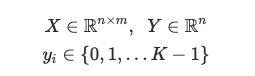
The goal now, is to estimate the probability of the class label taking on each of the K different possible values, i.e. P(y=k|x) for each k = 0, …, K-1. Therefore the prediction function will output a K-dimensional vector whose elements sum to 1, to give the K estimated probability.
Specifically, the hypothesis class now takes the form:

This is also known as multinomial logistic regression or softmax regression.
A note on dimensions —above we are looking at one example only, x is a m x 1 vector, y is an integer value between 0 and K-1, and let w(k) denote a m x 1 vector that represents the feature weights for the k-th class.
Each element of the output vector, takes the follow form:

This is known as the softmax function. The softmax turns arbitrary real values into probabilities. The outputs of the softmax function are always in the range [0, 1] and the summation in the denominator means all the terms add up to 1. Hence, they form a probability distribution. It can be seen as a generalization of the sigmoid function and in the binary case, the softmax function actually simplifies to the sigmoid function (try to prove this for yourself!)
For convenience, we specify the matrix W to denote all the parameters of the model. We concatenate all the w(k) vectors into columns so that the matrix W has dimension m x k.
As in the binary case, our goal in training is to learn the W values that minimize the cross entropy loss function (an extension of the binary formula).
We can think of logistic regression as a fully connected, single layer neural network followed by the softmax function.
The input layer contains a neuron for each feature (and potentially one neuron for a bias term). In the binary case, the output layer contains 1 neuron. In the multi-class case, the output layer contains a neuron for each class.
In fact, the traditional logistic regression and neural network formulations are equivalent. This is easiest to see in code — we can show that the NumPy implementation of the original formulas is equivalent to specifying a neural network in PyTorch. To illustrate, we’ll use examples from the Iris dataset.
The Iris dataset is a very simple dataset to demonstrate multi-class classification. There are 3 classes (encoded as 0, 1, 2) representing the type of iris flower (setosa, versicolor and virginica). There are 4 real-valued features for the length and width of both the plant sepal and petal.

Here is how we load and shuffle the Iris dataset using tools from the sci-kit learn datasets library:
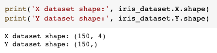
Let’s inspect the dataset dimensions:

There are 150 samples — in fact we know there are 50 samples of each class. Now, let’s pick two specific examples:
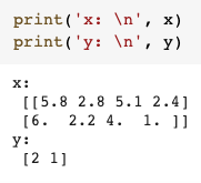
Above we see that, x has dimensions 2 x 4, because we have two examples and each example has 4 features. y has 2 x 1 values because we have two examples and each example has a label that could be 0, 1, 2 where each number represents the name of the class (versicolor, setosa, virginica).
Now we’ll create the weight parameters that we want to learn w. Since we have 4 features for each of the 3 classes, the dimension of w has to be 4 x 3.
Note: for simplicity, we’re looking only at the features and have not included a bias term here. Now we have,
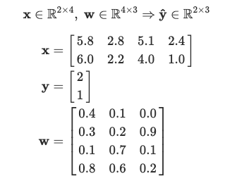
According to the logistic regression formula, we first compute z = xw. The shape of z is 2 x 3, because we have two samples and three possible classes. These raw scores need to be normalized into probabilities. We do this by applying the softmax function across each row of z.
Thus the final output y_hat has the same shape as z but now each row sums to 1 and each element of the row gives the probability of that column index as the predicted class.
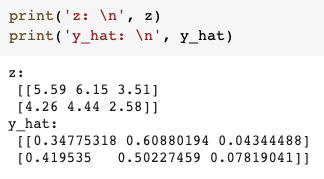
In the example above, the largest number in row 1 of y_hat is 0.6 which gives the second class label (1) as the predicted class. And for the second row, the predicted class is also 1, but with probability 0.5. In fact, in the second row, label 0 has also has a high probability of 0.41.
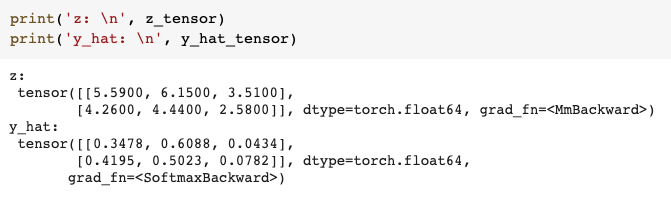
Now let’s implement the exact same thing but in PyTorch.
First we’ll need to convert our NumPy arrays to PyTorch Tensors.
Then define the linear layer and softmax activation function of the neural network.
PyTorch automatically initializes random weights so I explicitly replace the weights with the same weight matrix that we used above.
Now we calculate the output of this one layer neural network and see that it’s exactly the same as above.
This step above is called the forward pass (calculating the outputs and loss) when training a neural network the learn the optimal W. It is followed by the backward pass. During the backward pass, we calculate the gradient of the loss with respect to each weight parameter using the backpropagation algorithm (essentially, the chain rule) (link). Finally, we use the gradient descent algorithm to update the values of each of the weights. This constitutes one iteration. We repeat these steps, iteratively updating the weights, until the model converges or some stopping criteria is applied.
As you see, the outputs are the same whether you’re using NumPy or a neural network library like PyTorch. However, PyTorch uses tensor data-structures instead of NumPy arrays which are optimized for fast performance on hardware accelerators like GPUs and TPUs. Thus, this allows for a scalable implementation of logistic regression.
A second advantage of using PyTorch is that we can use automatic differentiation to efficiently and automatically calculate these gradients.
Although it’s simple to implement a simple logistic regression example as I just did, it becomes very difficult to distribute data batches and training on multiple GPUs/TPUs across many machines correctly.
However, by using PyTorch Lightning, I have implemented a version that handles all of these details and released it in the PyTorch Lightning Bolts library. This implementation makes it trivial to customize and train this model on any dataset.
pip install pytorch-lightning-bolts
We specify the number of input features, the number of classes and whether to include a bias term (by default this is set to true). For the Iris dataset, we would specify in_features=4 and num_classes=3. You can also specify a learning rate, L1 and/or L2 regularization.
Let’s continue with the Iris dataset as an example:
What you see above is how you load data in PyTorch using something called a Dataset and DataLoader. A Dataset is just a collection of examples and labels in PyTorch tensor format.
And a DataLoader is helps to efficiently iterate over batches (or subsets) of the Dataset. The DataLoader specifies things like the batch size, shuffle and data transforms.
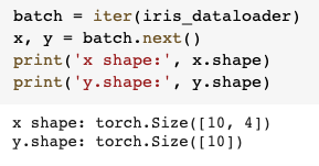
If we iterate over one batch in the DataLoader, we see that x and y both contain 10 samples, since we specified a batch size of 10.
DataModule:
In most approaches however we also need a training, validation and test splits of the data. With PyTorch Lightning, we have an extremely convenient class called a DataModule to automatically calculate these for us.
We use the SklearnDataModule — input any NumPy dataset, customize how you would like your dataset splits and it will return the DataLoaders for you to feed to your model.
A DataModule is nothing more than just a collection of a train DataLoader, validation DataLoader and test DataLoader. In addition to that, it allows you to fully specify and combine all your data preparation steps (like splits or data transforms) for reproducibility.
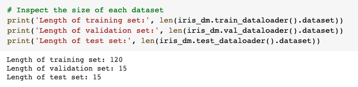
I’ve specified splitting the data into 80% train, 10% validation, 10% test but can also pass in your own validation and test datasets (as NumPy arrays) if you would like to use your own custom splits.
Say you have a custom test set with 20 samples and would like to use 10% of the training set for validation:
Splitting your data is good practice but completely optional — just set either or both the val_split and test_split to 0 if you don’t want to use a validation or test set.
Now that we have the data, let’s train our logistic regression model on 1 GPU. Training will start when I call trainer.fit (line 6). We can call trainer.test to see the model’s performance on our test set:
Our final test set accuracy is 100% — which is only something we get to enjoy with perfectly separably toy datasets like Iris.
Since I’m training this on a Colab notebook with 1 GPU, I’ve specified gpus=1 as an argument to the Trainer — however training on multiple hardware accelerators of any type is as simple as:
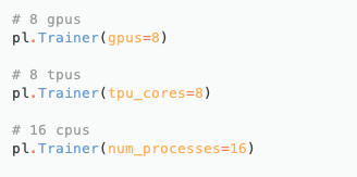
PyTorch Lightning deals with all the gritty details of distributed training behind the scenes so that you can focus on the model code.
Training on GPUs and TPUs is useful when running on large datasets. For small datasets, like Iris, hardware accelerators don’t make much of a difference.
For example, the original MNIST dataset of handwritten digits contains 70,000 images of 28*28 pixels each. That means that the input feature space has dimension 784, and K = 10 different classes in the output space. In fact, implementations in Sci-kit Learn don’t use the original dataset, instead downsampled images of only 8*8 pixels are used.

Given 785 features (28*28 + 1 for bias) and 10 classes, this means that our model has 7,850 weights that we’re learning (!).
Bolts conveniently has a MNISTDataModule that downloads, splits and applies that standard transforms like image normalization to the MNIST digit images.
Again we train using 1 GPU and see that the final test set accuracy (on 10,000 unseen images) is 92%. Pretty impressive!
Given the efficiency of PyTorch and the convenience of PyTorch Lightning, we could even scale this logistic regression model to train on massive datasets, like ImageNet, containing millions of samples.
If you’re interested in learning more about Lightning/Bolts I’d recommend looking at these resources:
Hopefully this guide showed you exactly how to get started. The easiest way to start is to run the Colab notebook with all the code examples we’ve looked at already.
You can try it yourself by just installing bolts and playing around! It includes different datasets, models, losses and callbacks you can mix and match, subclass, and run on your own data.
pip install pytorch-lightning-bolts
Or check out PyTorch Lightning Bolts.

The Ultimate Pytorch Research Framework