

Welcome to this beginner friendly guide to object detection using EfficientDet. Similarly to what I have done in the NLP guide (check it here if you haven’t yet already), there will be a mix of theory, practice, and an application to the global wheat competition dataset.
This will be a very long notebook, so use the following table of content if necessary. Grab something to drink and enjoy!
One last thing before I start, I have benefited immensely from the following two notebooks:
With these shoutouts out of the way, let’s start.
Computer vision went through a fast cycle of innovations and improvements starting in 2012 with the AlexNet network revolution.
Indeed, this was according to many one of the moments that launched again the field of deep learning from the last “AI winter”: for the first time, it was possible to train neural networks unsing large datasets and lots of compute (well according to 2012’s standards anyway :p).
This is what made the model achive state of the art performance on ImageNet. Indeed, it has achieved in 2012 a top-5 error of 15.3% which was 10% better than pervious year’s performance (the lower, the better).
So, what does this network contain?
The AlexNet network is quite simple: different CNN layers followed by max-pooling then a fully-connected layer.
Fast forward to 2020, a lot of things happened and the performances kept improving year after year: ImageNet is now considered a “solved” (kind of in most cases at least) dataset. In fact, it has been solved since at least 2015 with the introduction of the ResNet model, i.e. getting performance better than human-level for the first time (see the graph below).

To read more about what happened over the last years in the field of deep learning, check the following blog post
Most of these systems share similar architectures and modern “tips” to make them work best.
In what follows, I will detail some of what makes the modern computer vision ecosystem.
Here we go!
Before focusing on object detection, let’s move one step back and explore the modern computer vision landscape.
The first step was making CNNs work: that’s roughly what happened around 2012 and has been improved ever since as discussed in the previous section.
Then, the idea was to make the networks deeper to get better performances. Two main problems appeared then:
To solve these issues, few interesting ideas were introduced. As stated by Karpathy in one talk (haven’t found the link yet, if you know it, please share in the comments): “more zeros, better performance”. What does that mean? In short, more 0s everywhere in the network:
Thus less parameters.
Something else happened: code discovery, sharing, and reproducibility got better. I don’t have any data to back this claim but that’s what I have observed through experience. For instance, papers with code is probably the best place to look for a code implementation.
Also, the code ecosystem got much better. Among the recent code libraries and tools:
Finally, some of the recent research trends:
All these things make the modern-days computer vision ecosystem. Let’s now move to the subfield of object detection.
We will mainly focus on three similar detection tasks (from simpler to more complex):
Object detection is the easiest one. It consists in placing bounding boxes around detected objects. The two remaining tasks are best described in the image below:
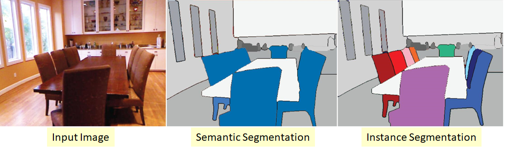
All three tasks share the following thing: given an object the aim is to locate some pixels that identify it:

The two most popular ways to annotate a bounding box. Left for the reader: how to move from one to the other?
Now that we are more familiar with the general detection tasks, we can move to object detection.
What is object detection?
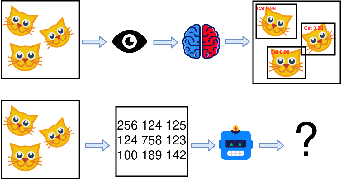
For humans, this is a straightforward question: given an image and a label, draw a bounding box around the detected objects. In other words, it is localization plus classification of objects.
However, translating this task into an algorithm is on another level of hard. Indeed, where do you even start?
I also like this definition from paperswithcode:
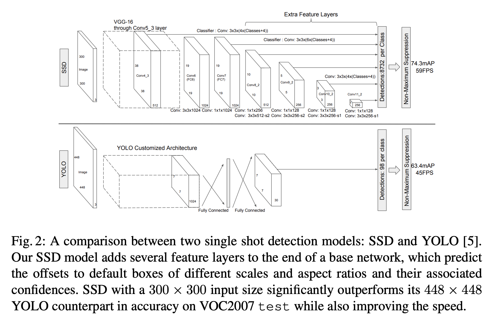
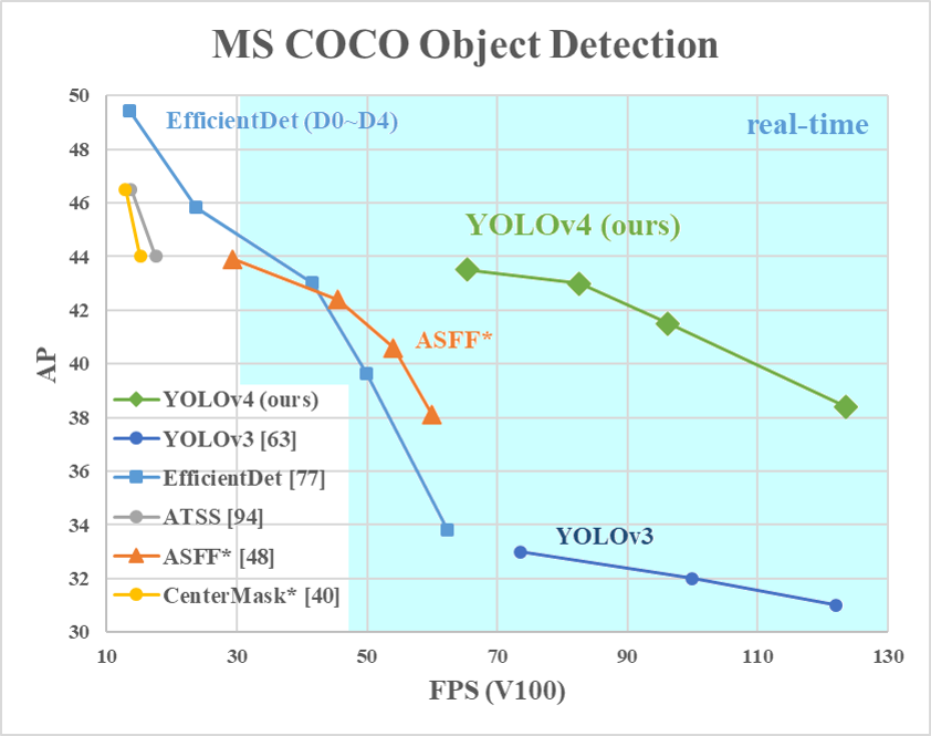
Object detection is the task of detecting instances of objects of a certain class within an image. The state-of-the-art methods can be categorized into two main types: one-stage methods and two stage-methods. One-stage methods prioritize inference speed, and example models include YOLO, SSD and RetinaNet. Two-stage methods prioritize detection accuracy, and example models include Faster R-CNN, Mask R-CNN and Cascade R-CNN. The most popular benchmark is the MSCOCO dataset. Models are typically evaluated according to a Mean Average Precision metric.
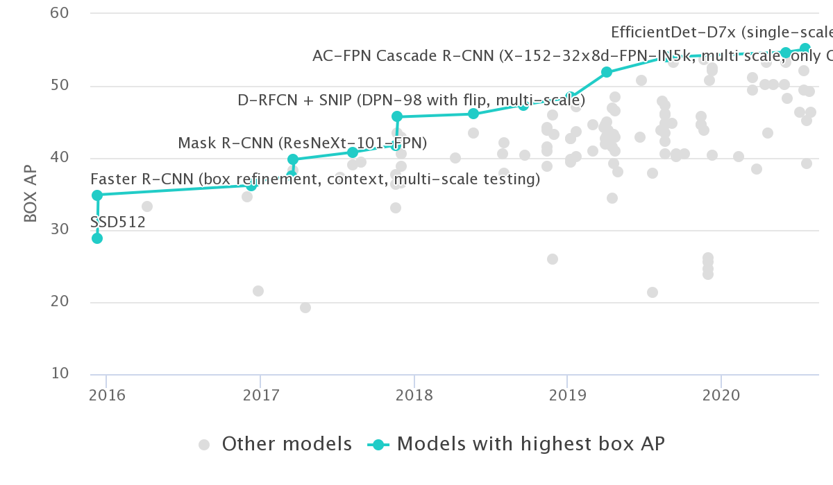
Fortunately, we don’t need to really understand what goes inside our brains. It appears that deep learning models are very good at that. Indeed, given the latest ImageNet and COCO benchmarks, deep learning models are beating human-level performance: that was the case on the ImageNet dataset since 2015 and that’s the case for the COCO dataset since .
So, the next question is: how to design a good neural network for object detection?
Let’s have a look at the most common techniques to have a feel for what works. From Wikipedia’s object detection page:
We can also add EfficientDet ;). Well this list isn’t very informative, is it? Based on my own experience (basically reading a lot of blog posts and papers), there are two major families:
R-CNN and its “cousins” fall into the first family of models. In contrast to the R-CNN family, SSD, YOLO, RetinaNet, CeneterNet and EfficientDet fall into the faster, one step family.
Finally, to learn more about these two families of models, check this blog post and this slides deck telling a brief history of object detection.
Let’s explore further this rich ecosystem of models.
As stated above, it seems that deep learning models, particularly convolutional ones are very good at image processing tasks, and in particular object detection. We won’t explore why this is the case so feel free to explore this subject on your own. One possible explanation is that deep neural networks are good at distilling features from noisy inputs and this can be explained by the information bottleneck theory.
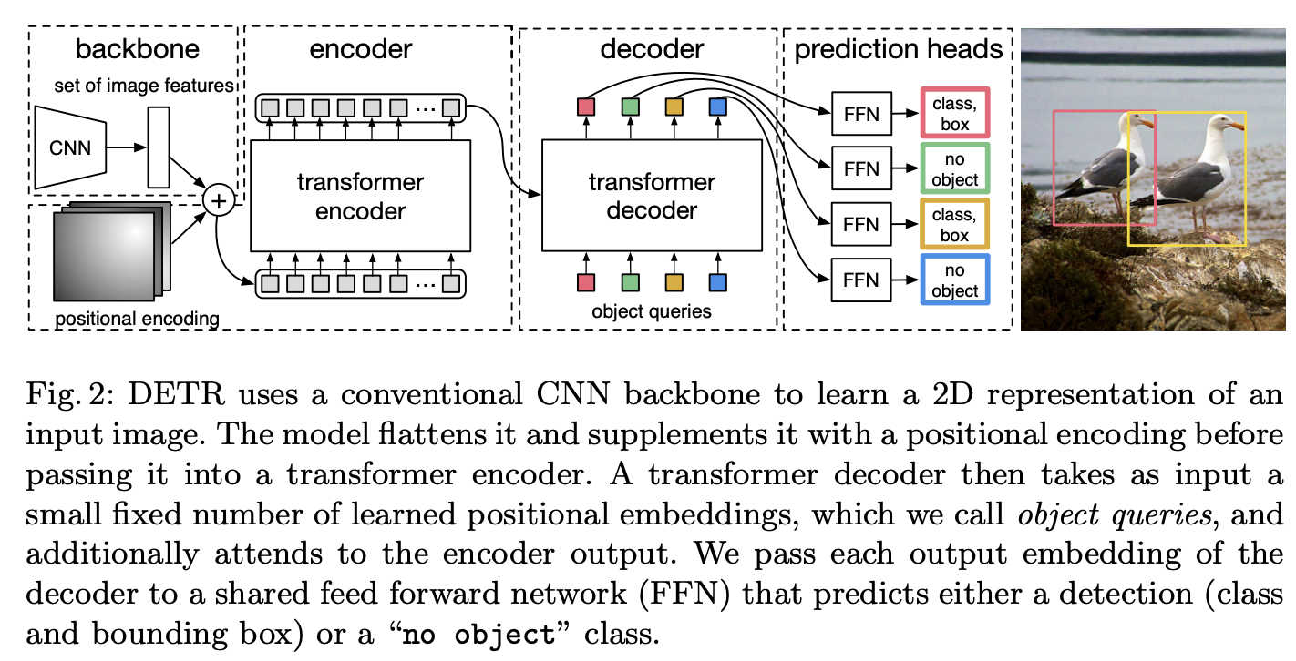
Instead, let’s explore some SOTA (state-of-the-art) models and see what they have in common:
To dig deeper, here are some more details:


That was a lot of new concepts to groak, so as a reward, here is an approximate timeline: in red the one step models, and green the two steps ones. Notice that FPN doesn’t have a category since it is used in both:

That’s enough general architecture for now! In the remaining parts, we will be focusing on the EfficienDet family of models, more specifically on the following Pytorch implementation.
What is EfficientDet and how does it work?
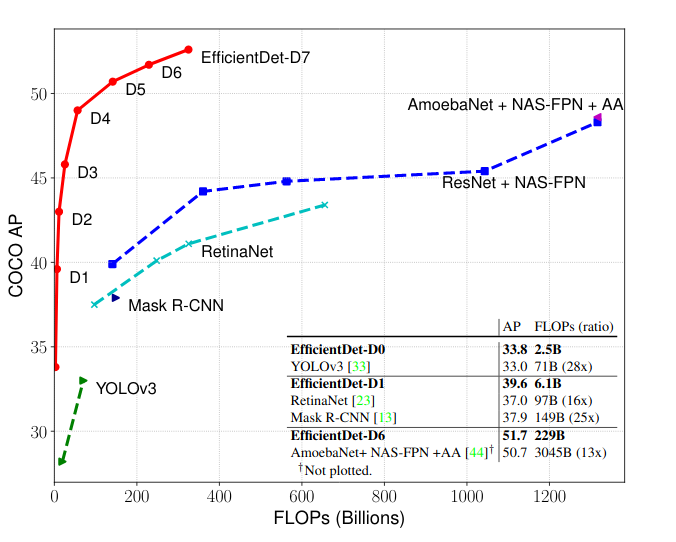
In short, it is a recent (first submitted at the end of 2019, accepted in CVPR in 2020) very efficient (surprise surprise) object detection model.
In more details, it is a family of models designed by researchers from Google brain. The interesting thing is that some parts of it were designed using automatic architecture search, i.e. there was a meta-model that was trained to find the best hyper-parameters of the trained model automatically. Let’s dive in more details.
First, let’s start with the model’s architecture:
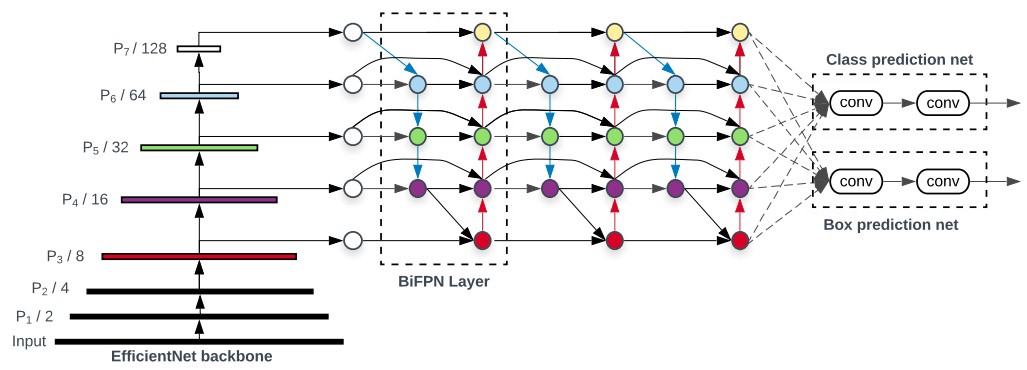
As you can see, there are 3 main building blocks:
In more details, we have:
To experiment with the model and learn more, check this colab notebook, the original paper, and the original implementation.
In the following sections, we will explore each part in more details. Let’s go!
This is the first part of the architecture. It uses the EfficientNet architecture and includes pre-trained weights.
Here is a look at the overall architecture:

As you can see, the interesting thing is that many elements of the model have been optimized using neural automatic search: width, depth, number of channels, and resolution.
To learn more about this EfficientNet backbone, read the original paper here, the blog post, and the implementation here (from the efficientdet repo).
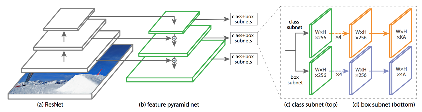
Once we have a classification network, one important question to ask is: how to move from the classification model to an object detection one? This is cleverly solved by using features maps (i.e. intermediate learned representations). Another question is how to detect multiple objects having different sizes (for example a small cat and a car on the same image)? This is solved by taking features maps having different sizes.
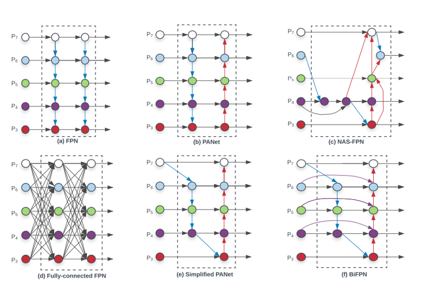
In most modern object detection architectures, both problems are solved at once using an FPN layer. BiFPN, as its name indicates, builds upon the ideas of the FPN layer and adds one simple idea: instead of simply aggregating the different representations in a top-down fashion, it takes the PANet approach (i.e. top-down and bottom-up connections) and optimizes cross-scale connections.
One last trick is to use a weighted feature fusion instead of the unweighted FPN approach (the weights are learned as well) and normalize these weights using a fast normalization procedure (i.e. normalize by the sum instead of using softmax). Here is one example of a BiFPN computation from the paper:
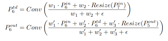
All these tricks make the BiFPN layer both efficient and accurate. We will see one additional trick applied in the next and last section. Check the following graph to learn more about other FPN variations (including PANet and BiFPN):
Finally, to learn more about FPN and BiFPN, check the papeswithcode page, this blog post, and this one as well.
Let’s move to the next step: the prediction networks.
The third ingredient to the mix is the two heads network:
Each of the two networks take as input all the outputs of the previous BiFPN layer. Then we have two fully-connected layers before getting the final values. As simple as that!
We close this section with the last trick: compound scaling.
One last ingredient to the mix is how the network is scaled. Indeed, this is a trick often used to improve the performance of networks. The most common way to do it is to scale the backbone’s width and depth.
In the EfficientDet model, the EffincientNet backbone is scaled reusing the same values in the original network. The interesting additional thing is the scaling of the BiFPN and prediction networks. In fact, instead of using only one BiFPN and one prediction networks, these components are repeated. Finally, width ($W$), depth ($D$), and input resolution ($R$) in the different sections are scaled using one single parameter $\phi$ in this fashion:
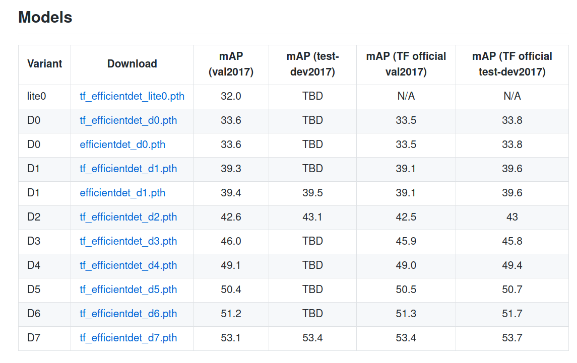
Here is the table for the different EfficientDet variants: the bigger $\phi$ is, the bigger the model:

To finish this section, notice that the $1.35$ value in the first equation has been optimized using grid search (i.e. different values are tested and the one giving the best score is selected) over ${1.2, 1.25, 1.3, 1.35, 1.4, 1.45}$ values.
That’s it for the model’s architecture. Time to move to the application!
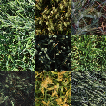
Now that the theory makes (hopefully) more sense, let’s move to the application side of things. In the above figure, you can see a patch of wheat heads.
That’s the competition’s banner and that’s what we are predicting: finding the bounding boxes of wheat heads.
As stated in the introduction, we will be using the EfficientDet model introduced above.
Here is a rough sketch of the plan:
As you have guessed it, the task of this competition is to predict the bounding boxes of wheat heads in different images. The images have a varying number of wheat heads, colors, orientations, and so on making the task more challenging.
To further understand the task, let’s explore the wheat images and the associated bounding boxes:


The evaluation metric for object detection is quite tricky (when compared to object classification). Here is how it is computed:
If this explanation isn’t clear enough, check the following paper detailing object detection metrics and how they are computed.
Enough with theory, let’s move to the implementation!
Similarly the the previous NLP notebook, I will be using Pytorch Lightning to implement the model. For that, we will start by defining the model part then move to the data processing, evaluation, and prediction.
Let’s get started!
To make things easier (DRY principle), I will be using the following EfficientDet model.
To create the model, the code snippet is quite simple (D5 EfficientDet here but you can use the one that suits your needs):
from effdet import get_efficientdet_config, EfficientDet, DetBenchTrain
from effdet.efficientdet import HeadNet
def get_train_efficientdet():
# Get the model's config
config = get_efficientdet_config("tf_efficientdet_d5")
# Create the model
net = EfficientDet(config, pretrained_backbone=False)
# Load pretrained EfficientDet weights
checkpoint = torch.load("path/to/weights")
net.load_state_dict(checkpoint)
# Change the number of classes to 1 (only predicting wheat)
config.num_classes = 1
config.image_size = 256
# Add the head with the updated parameters
head = HeadNet(
config,
num_outputs=config.num_classes,
norm_kwargs=dict(eps=0.001, momentum=0.01),
)
# Attach the head
net.class_net = head
return DetBenchTrain(net, config)
In what follows, we will use this code snippet to create the model. Next, let’s see how we can create a WheatDataset: if you aren't familiar with Pytorch's Dataset concept, check it here.
Before I start, notice that some of the code (mostly?) is inspired from this notebook, so go check it out and thank Peter for making it!
from torch.utils.data import DataLoader, Dataset
import torch
from PIL import Image
import albumentations as A
from albumentations.pytorch.transforms import ToTensorV2
import numpy as np
import pandas as pd
from pathlib import Path
# Using a small image size so it trains faster but do try bigger images
# for better performance.
IMG_SIZE = 256
def get_train_transforms():
return A.Compose(
[
A.RandomSizedCrop(min_max_height=(800, 800), height=IMG_SIZE, width=IMG_SIZE, p=0.5),
A.OneOf([
A.HueSaturationValue(hue_shift_limit=0.2, sat_shift_limit= 0.2,
val_shift_limit=0.2, p=0.9),
A.RandomBrightnessContrast(brightness_limit=0.2,
contrast_limit=0.2, p=0.9),
],p=0.9),
A.ToGray(p=0.01),
A.HorizontalFlip(p=0.5),
A.VerticalFlip(p=0.5),
A.Resize(height=256, width=256, p=1),
A.Cutout(num_holes=8, max_h_size=64, max_w_size=64, fill_value=0, p=0.5),
ToTensorV2(p=1.0),
],
p=1.0,
bbox_params=A.BboxParams(
format='pascal_voc',
min_area=0,
min_visibility=0,
label_fields=['labels']
)
)
def get_valid_transforms():
return A.Compose(
[
A.Resize(height=IMG_SIZE, width=IMG_SIZE, p=1.0),
ToTensorV2(p=1.0),
],
p=1.0,
bbox_params=A.BboxParams(
format='pascal_voc',
min_area=0,
min_visibility=0,
label_fields=['labels']
)
)
def get_test_transforms():
return A.Compose([
A.Resize(height=IMG_SIZE, width=IMG_SIZE, p=1.0),
ToTensorV2(p=1.0),
], p=1.0)
class WheatDataset(Dataset):
def __init__(self, df = None, mode = "train", image_dir = "", transforms=None):
super().__init__()
if df is not None:
self.df = df.copy()
self.image_ids = df['image_id'].unique()
else:
# Test case
self.df = None
self.image_ids = [p.stem for p in Path(image_dir).glob("*.jpg")]
self.image_dir = image_dir
self.transforms = transforms
self.mode = mode
def __getitem__(self, index: int):
image_id = self.image_ids[index]
# Could be one or many rows.
image = Image.open(f'{self.image_dir}/{image_id}.jpg').convert("RGB")
# Convert to Numpy array
image = np.array(image)
image = image / 255.0
image = image.astype(np.float32)
if self.mode != "test":
records = self.df[self.df['image_id'] == image_id]
area = records["area"].values
area = torch.as_tensor(area, dtype=torch.float32)
boxes = records[["x", "y", "x2", "y2"]].values
# there is only one class, so always 1.
labels = torch.ones((records.shape[0],), dtype=torch.int64)
# suppose all instances are not crowd.
iscrowd = torch.zeros((records.shape[0],), dtype=torch.int64)
target = {}
target['boxes'] = boxes
target['labels'] = labels
# target['masks'] = None
target['image_id'] = torch.tensor([index])
target['area'] = area
target['iscrowd'] = iscrowd
# These are needed as well by the efficientdet model.
target['img_size'] = torch.tensor([(IMG_SIZE, IMG_SIZE)])
target['img_scale'] = torch.tensor([1.])
else:
# test dataset must have some values so that transforms work.
target = {'cls': torch.as_tensor([[0]], dtype=torch.float32),
'bbox': torch.as_tensor([[0, 0, 0, 0]], dtype=torch.float32),
'img_size': torch.tensor([(IMG_SIZE, IMG_SIZE)]),
'img_scale': torch.tensor([1.])}
if self.mode != "test":
if self.transforms:
sample = {
'image': image,
'bboxes': target['boxes'],
'labels': labels
}
if len(sample['bboxes']) > 0:
# Apply some augmentation on the fly.
sample = self.transforms(**sample)
image = sample['image']
boxes = sample['bboxes']
# Need yxyx format for EfficientDet.
target['boxes'] = torch.stack(tuple(map(torch.tensor, zip(*boxes)))).permute(1, 0)
else:
sample = {
'image': image,
'bbox': target['bbox'],
'cls': target['cls']
}
image = self.transforms(**sample)['image']
return image, target
def __len__(self) -> int:
return len(self.image_ids)
So, what have we done above?
Let’s check that this implementation works by sampling from the WheatDataset. Before that one small detour to process the labels' DataFrame and add some useful metadata such as the bounding box area and the lower corner's coordiantes.
# Some processing to add some metadata to the labels DataFrame
train_labels_df = pd.read_csv("../input/global-wheat-detection/train.csv")
train_labels_df['bbox'] = train_labels_df['bbox'].apply(eval)
x = []
y = []
w = []
h = []
for bbox in train_labels_df['bbox']:
x.append(bbox[0])
y.append(bbox[1])
w.append(bbox[2])
h.append(bbox[3])
processed_train_labels_df = train_labels_df.copy()
processed_train_labels_df["x"] = x
processed_train_labels_df["y"] = y
processed_train_labels_df["w"] = w
processed_train_labels_df["h"] = h
processed_train_labels_df["area"] = processed_train_labels_df["w"] * processed_train_labels_df["h"]
processed_train_labels_df["x2"] = processed_train_labels_df["x"] + processed_train_labels_df["w"]
processed_train_labels_df["y2"] = processed_train_labels_df["y"] + processed_train_labels_df["h"]# Create stratified folds, here using the source.
# This isn't the most optimal way to do it but I will leave it to you
# to find a better one. ;)
from sklearn.model_selection import StratifiedKFold
skf = StratifiedKFold(n_splits=5)
for fold, (train_index, valid_index) in enumerate(skf.split(processed_train_labels_df,
y=processed_train_labels_df["source"])):
processed_train_labels_df.loc[valid_index, "fold"] = foldprocessed_train_labels_df.sample(2).T# We need to set a folder to get images
TRAIN_IMG_FOLDER = "../input/global-wheat-detection/train"
# This is the transforms for the training phase
train_transforms = get_train_transforms()
train_dataset = WheatDataset(
processed_train_labels_df, mode="train", image_dir=TRAIN_IMG_FOLDER, transforms=train_transforms
)
image, target = train_dataset[0]print(image)
print(target)import matplotlib.pylab as plt
from PIL import Image, ImageDraw
import pandas as pd
from pathlib import Path
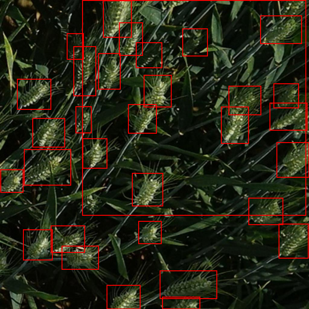
def plot_image_with_bboxes(img_id, df):
img_path = Path(TRAIN_IMG_FOLDER + f"/{img_id}.jpg")
img = Image.open(img_path)
draw = ImageDraw.Draw(img)
bboxes = df.loc[lambda df: df["image_id"] == img_id, "bbox"]
# The box contains the upper left corner (x, y) coordinates then width and height.
# So we need to change these to (x1, y1) and (x2, y2) where they are the upper
# left and lower right corners
for bbox in bboxes:
x, y, w, h = bbox
transformed_bbox = [x, y, x + w, y + h]
draw.rectangle(transformed_bbox, outline="red", width=3)
return img
plot_image_with_bboxes("00333207f", processed_train_labels_df)
Looks fine, awesome! Time to move to the training pipeline.
Alright, time to build a model. For that, we will be using the belvoed Pytorch Lightning. As usual, we will start with the model building block then add the processing steps. As a first step, we install the Pytorch Lightning library using pip: pip install pytorch_lightning.
Next, we install the efficientdet library, again using pip: pip install effdet. Notice that the efficientdet library needs timm (PyTorch Image Models library). For that, we also need to run: pip install timm. There is finally omegaconf and pycocotools (same using pip).
!pip install pytorch_lightning
!pip install effdet --upgrade
!pip install timm
!pip install omegaconf
!pip install pycocotools
Everything is set, time to create the EfficientDet model using the code snippet presented above (the get_train_efficientdet function).
import torch
from effdet import get_efficientdet_config, EfficientDet, DetBenchTrain
from effdet.efficientdet import HeadNet
def get_train_efficientdet():
config = get_efficientdet_config('tf_efficientdet_d5')
net = EfficientDet(config, pretrained_backbone=False)
checkpoint = torch.load('../input/efficientdet/efficientdet_d5-ef44aea8.pth')
net.load_state_dict(checkpoint)
config.num_classes = 1
config.image_size = IMG_SIZE
net.class_net = HeadNet(config, num_outputs=config.num_classes, norm_kwargs=dict(eps=.001, momentum=.01))
return DetBenchTrain(net, config)from pytorch_lightning import LightningModule
class WheatModel(LightningModule):
def __init__(self, df, fold):
super().__init__()
self.df = df
self.train_df = self.df.loc[lambda df: df["fold"] != fold]
self.valid_df = self.df.loc[lambda df: df["fold"] == fold]
self.image_dir = TRAIN_IMG_FOLDER
self.model = get_train_efficientdet()
self.num_workers = 4
self.batch_size = 8
def forward(self, image, target):
return self.model(image, target)
# Create a model for one fold.
model = WheatModel(processed_train_labels_df, fold=0)modelfrom torch.utils.data import Dataset, DataLoader, RandomSampler, SequentialSampler
def collate_fn(batch):
return tuple(zip(*batch))
# Let's add the train and validation data loaders.
def train_dataloader(self):
train_transforms = get_train_transforms()
train_dataset = WheatDataset(
self.train_df, image_dir=self.image_dir, transforms=train_transforms
)
return DataLoader(
train_dataset,
batch_size=self.batch_size,
sampler=RandomSampler(train_dataset),
pin_memory=False,
drop_last=True,
collate_fn=collate_fn,
num_workers=self.num_workers,
)
def val_dataloader(self):
valid_transforms = get_train_transforms()
valid_dataset = WheatDataset(
self.valid_df, image_dir=self.image_dir, transforms=valid_transforms
)
valid_dataloader = DataLoader(
valid_dataset,
batch_size=self.batch_size,
sampler=SequentialSampler(valid_dataset),
pin_memory=False,
shuffle=False,
collate_fn=collate_fn,
num_workers=self.num_workers,
)
iou_types = ["bbox"]
# Had to comment these since the evaluation doesn't work yet.
# More on this in the next section.
# coco = convert_to_coco_api(valid_dataset)
# self.coco_evaluator = CocoEvaluator(coco, iou_types)
return valid_dataloader
WheatModel.train_dataloader = train_dataloader
WheatModel.val_dataloader = val_dataloaderdef training_step(self, batch, batch_idx):
images, targets = batch
targets = [{k: v for k, v in t.items()} for t in targets]
# separate losses
images = torch.stack(images).float()
targets2 = {}
targets2["bbox"] = [
target["boxes"].float() for target in targets
] # variable number of instances, so the entire structure can be forced to tensor
targets2["cls"] = [target["labels"].float() for target in targets]
targets2["image_id"] = torch.tensor(
[target["image_id"] for target in targets]
).float()
targets2["img_scale"] = torch.tensor(
[target["img_scale"] for target in targets]
).float()
targets2["img_size"] = torch.tensor(
[(IMG_SIZE, IMG_SIZE) for target in targets]
).float()
losses_dict = self.model(images, targets2)
return {"loss": losses_dict["loss"], "log": losses_dict}
def validation_step(self, batch, batch_idx):
images, targets = batch
targets = [{k: v for k, v in t.items()} for t in targets]
# separate losses
images = torch.stack(images).float()
targets2 = {}
targets2["bbox"] = [
target["boxes"].float() for target in targets
] # variable number of instances, so the entire structure can be forced to tensor
targets2["cls"] = [target["labels"].float() for target in targets]
targets2["image_id"] = torch.tensor(
[target["image_id"] for target in targets]
).float()
targets2["img_scale"] = torch.tensor(
[target["img_scale"] for target in targets], device="cuda"
).float()
targets2["img_size"] = torch.tensor(
[(IMG_SIZE, IMG_SIZE) for target in targets], device="cuda"
).float()
losses_dict = self.model(images, targets2)
loss_val = losses_dict["loss"]
detections = losses_dict["detections"]
# Back to xyxy format.
detections[:, :, [1,0,3,2]] = detections[:, :, [0,1,2,3]]
# xywh to xyxy => not necessary.
# detections[:, :, 2] += detections[:, :, 0]
# detections[:, :, 3] += detections[:, :, 1]
res = {target["image_id"].item(): {
'boxes': output[:, 0:4],
'scores': output[:, 4],
'labels': output[:, 5]}
for target, output in zip(targets, detections)}
# iou = self._calculate_iou(targets, res, IMG_SIZE)
# iou = torch.as_tensor(iou)
# self.coco_evaluator.update(res)
return {"loss": loss_val, "log": losses_dict}
def validation_epoch_end(self, outputs):
# self.coco_evaluator.accumulate()
# self.coco_evaluator.summarize()
# coco main metric
# metric = self.coco_evaluator.coco_eval["bbox"].stats[0]
# metric = torch.as_tensor(metric)
# tensorboard_logs = {"main_score": metric}
# return {
# "val_loss": metric,
# "log": tensorboard_logs,
# "progress_bar": tensorboard_logs,
# }
pass
def configure_optimizers(self):
return torch.optim.AdamW(self.model.parameters(), lr=1e-4)
WheatModel.training_step = training_step
# Had to comment these since the evaluation doesn't work yet. More on this
# in the next section.
# WheatModel.validation_step = validation_step
# WheatModel.validation_epoch_end = validation_epoch_end
WheatModel.configure_optimizers = configure_optimizers
That’s it, our WheatModel is ready now. Let's train it. For that, we will create a Trainer and set it to fast_dev_run=True for a quicker demo. Also, since it is in this mode, the Trainer doesn't automatically save the weights at the end (correct me if I am wrong of course) so we need to add a torch.save call at the end.
from pytorch_lightning import Trainer, seed_everything, loggers
seed_everything(314)
# Create a model for one fold.
# As an exercise, try doing it for the other folds and chaning the Trainer. ;)
model = WheatModel(processed_train_labels_df, fold=0)
logger = loggers.TensorBoardLogger("logs", name="effdet-b5", version="fold_0")
trainer = Trainer(gpus=1, logger=logger, fast_dev_run=True)
trainer.fit(model)
torch.save(model.model.state_dict(), "wheatdet.pth")
Believe it or not, this is a part where I struggled the most. This isn’t because of the tool but it was due to the code that I was using. Indeed, the evaluation part is tied to the torchvision repo and I haven't found a simple way to import it. Thus I needed to copy a lot of code as was done in artgor's notebook. I won't show this part since it is tedious and not very elegant. If you have found a better method, please share it with me in the comments section.
Another route I have tried is a similar one used here where they have cloned the torchvision part from the Pytorch’s repo then copying the necessary parts using cp (instead of manually doing it). I am sure it works eventually but I won’t do this here since the notebook is long enough already and I am being a little lazy. I will try to make this section work later on.
# Download TorchVision repo to use some files from
# references/detection
"""
!git clone https://github.com/pytorch/vision.git
!cd vision
!git checkout v0.3.0
!cp references/detection/utils.py ../
!cp references/detection/transforms.py ../
!cp references/detection/coco_eval.py ../
!cp references/detection/engine.py ../
!cp references/detection/coco_utils.py ../
"""
To finish this section, let’s make some predictions.
Mostly inspired (i.e. copied ;)) from here. Again, thanks Alex Shonenkov. I won’t go over the formatting step to make a proper submission file. Check the notebook if you want to learn about these final steps.
Also, in a better world, I would have made this part using Pytorch Lightning but I am little overwhelmed with this very lengthy notebook so it is enough for now. ;)
from effdet import DetBenchPredict
def get_test_efficientdet(checkpoint_path):
config = get_efficientdet_config('tf_efficientdet_d5')
net = EfficientDet(config, pretrained_backbone=False)
config.num_classes = 1
config.image_size=IMG_SIZE
net.class_net = HeadNet(config, num_outputs=config.num_classes,
norm_kwargs=dict(eps=.001, momentum=.01))
checkpoint = torch.load(checkpoint_path)
net.load_state_dict(checkpoint, strict=False)
net = DetBenchPredict(net, config)
return net
def make_predictions(model, images, score_threshold=0.22):
images = torch.stack(images).float()
predictions = []
targets = torch.tensor([1]*images.shape[0])
img_scales = torch.tensor(
[1 for target in targets]
).float()
img_sizes = torch.tensor(
[(IMG_SIZE, IMG_SIZE) for target in targets]
).float()
with torch.no_grad():
detections = model(images, img_scales, img_sizes)
for i in range(images.shape[0]):
pred = detections[i].detach().cpu().numpy()
boxes = pred[:,:4]
scores = pred[:,4]
indexes = np.where(scores > score_threshold)[0]
boxes = boxes[indexes]
boxes[:, 2] = boxes[:, 2] + boxes[:, 0]
boxes[:, 3] = boxes[:, 3] + boxes[:, 1]
predictions.append({
'boxes': boxes[indexes],
'scores': scores[indexes],
})
return predictionsTEST_IMG_FOLDER = "../input/global-wheat-detection/test"
test_model = get_test_efficientdet("wheatdet.pth")
test_dataset = WheatDataset(
None, mode="test", image_dir=TEST_IMG_FOLDER, transforms=get_test_transforms()
)
image, _ = test_dataset[0]
predictions = make_predictions(test_model, [image])predictions
Hurray, we have predictions!
Before finishing this (lengthy) notebook, I wanted to talk about few advanced concepts to get better results particularly for object detection but they do work for many computer vision tasks. As you might have seen, the results you get from training the model presented above are quite good but not enough to be competitive. Indeed, winning solutions used EfficientDet augmented with few more tricks.
Here are some advanced concepts to get you better results:
Let’s start with mosaic augmentation.
This technique concists in stitching together different images to form a bigger one. The more diverse the images, the better it is. If you are curious, you can check an example of how to use it here from the winning competition solution. The following example is extracted from the same post, thanks again to DungNB for the write-up!
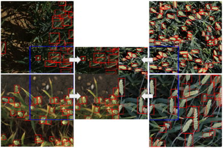
Here is a simple explanation using cat images:

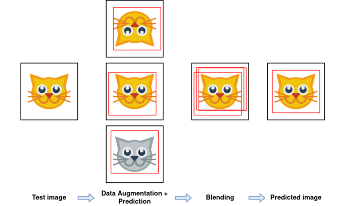
TTA, short for test-time augmentation, is a popular technique for getting better performance for computer vision tasks and you will often encounter it when doing Kaggle computer vision competitions.
How does it work?
The basic idea is quite simple:
For the augmentation step, horizantal and vertical flips are quite common strategies for TTA. Notice that since this step happens during inference time and since code competitions have time limits, you can’t use a lot of augmentation. 2 or 3 additional images per original test one is more than enough. Finally, for object detection, since there is a bounding box to predict, the augmentation step should preserve the shape of the bounding box. Thus some augmentations aren’t allowed (for instance 90 degrees rotations).
To finish this section, here is an illustration (again, using cats :p)
If you are accustomed to object detection tasks and challenges, you may have heard about NMS (short for non-maximum suppresion). Here is a short description of its pseudo-code:
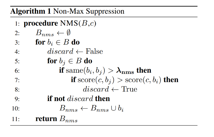
Check this post for more details (the figure above is from it).
This technique is used to merge many boxes (called proposals) from one model and can be used to merge the results of many models as well.
Here, we will go over another technique called weighted-boxes fusion or (WBF in short).
To get started, you can check the Github implementation here, the paper or this great notebook again from Alex Shonenkov, so thanks!
So how does it work and how is it different? Let’s have a look at the following schema (from the WBF paper)
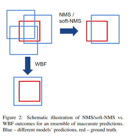
If you may have noticed, the WBF algorithm “made” a bounding box that isn’t any of the proposed ones whereas NMS came up with one from the proposals. Indeed, that’s one of the big differences between the two: how different proposals are merged. For the WBF case, the main objective is to compute a new confidence score C from existing confidence scores and then use it to compute the blended bounding box coordinates and confidence as a weighted mean (or other functions).
Finally, if you want even more blending techniques, you can explore these techniques:


That’s it for today. If you made it this far, congratulations!
By now, you should have acquired basic knowledge of object detection and computer vision more generally, you can now go and build models. Congratulations on gaining a new (super) power!
Stay tuned for the next notebook and in the meantime, happy kaggling!
Going further, check these resources to expand your understanding:
The Ultimate Pytorch Research Framework