

This article looks at using PyTorch Lightning for the exciting domain of Reinforcement Learning (RL). Here we are going to build a standard Deep Q Network (DQN) model using the classic CartPole gym environment to illustrate how to start using Lightning to build your RL models.
In this article we will cover:
If you would like to jump straight to the code you can find the example in the PyTorch Lightning examples page or check out the interactive colab notebook by clicking the colab icon below!

Lightning is a recent PyTorch library that cleanly abstracts and automates all the day to day boilerplate code that comes with ML models, allowing you to focus on the actual ML part (the fun part!) . If you haven’t already, I highly recommend you check out some of the great articles published by the Lightning team
As well as automating boilerplate code, Lightning acts as a type of style guide for building clean and reproducible ML systems.
This is very appealing for a few reasons:
Before we get into the code, lets do a quick recap of what a DQN does. A DQN learns the best policy for a given environment by learning the value of taking each action A while being in a specific state S. These are known as Q values.
Initially the agent has a very poor understanding of its environment as it hasn’t had much experience with it. As such, its Q values will be very inaccurate. However, over time as the agent explores its environment, it learns more accurate Q values and can then make good decisions. This allows it improve even further, until it eventually converges on an optimal policy (ideally).
Most environments of interest to us like modern video games and simulations are far too complex and large to store the values for each state/action pair. This is why we use deep neural networks to approximate the values.
The general life cycle of the agent is described below:
That’s a high level overview of what the DQN does. For more information there are lots of great resources on this popular model out there for free such as the PyTorch example. If you want to learn more about reinforcement learning in general, I highly recommend Maxim Lapan’s latest book Deep Reinforcement Learning Hands On Second Edition

Lets take a look at the parts that make up our DQN
Model: The neural network used to approximate our Q values
Replay Buffer: This is the memory of our agent and is used to store previous experiences
Agent: The agent itself is what interacts with the environment and the replay buffer
Lightning Module: Handles all the training of the agent
For this example we can use a very simple Multi Layer Perceptron (MLP). All this means is that we aren’t using anything fancy like Convolutional or Recurrent layers, just normal Linear layers. The reason for this is due to the simplicity of the CartPole environment, anything more complex than this would be overkill.
The replay buffer is fairly straight forward. All we need is some type of data structure to store tuples. We need to be able to sample these tuples and also add new tuples. This buffer is based off Lapins replay buffer found here as it is the cleanest and fastest implementation I have found so far. That looks something like this
But we aren’t done. If you have used Lightning before you know that its structure is based around the idea of DataLoaders being created and then used behind the scenes to pass mini batches to each training step. It is very clear how this works for most ML systems such as supervised models, but how does it work when we are generating our dataset as we go?
We need to create our own IterableDataset that uses the continuously updated Replay Buffer to sample previous experiences from. We then have mini batches of experiences passed to the training_step to be used to calculate our loss, just like any other model. Except instead of containing inputs and labels, our mini batch contains (states, actions, rewards, next states, dones)
You can see that when the dataset is being created, we pass in our ReplayBuffer which can then be sampled from to allow the DataLoader to pass batches to the Lightning Module.
The agent class is going to handle the interaction with the environment. There are 3 main methods that are carried out by the agent
get_action: Using the epsilon value passed, the agent decides whether to use a random action, or to take the action with the highest Q value from the network output.
play_step: Here the agent carries out a single step through the environment with the action chosen from get action. After getting the feedback from the environment, the experience is stored in the replay buffer. If the environment was finished with that step, the environment resets. Finally, the current reward and done flag is returned.
reset: resets the environment and updates the current state stored in the agent.
Now that we have our core classes for our DQN set up we can start looking at training the DQN agent. This is where Lightning comes in. We are going lay out all of our training logic in a clean and structured way by building out a Lightning Module.
Lightning provides a lot of hooks and override-able functions allowing for maximum flexibility, but there are 4 key methods that we must implement to get our project running. That is the following.
With these 4 methods populated we can make pretty train any ML model we would encounter. Anything that requires more than these methods fit in nicely with the remaining hooks and callbacks within Lightning. For a full list of these available hooks, check out the Lightning docs . Now, lets look at populating our Lightning methods.
First we need to initialize our environment, networks, agent and the replay buffer. We also call the populate function which will fill the replay buffer with random experiences to begin with (The populate function is shown in the full code example further down).

All we are doing here is wrapping the forward function of our primary DQN network.

Before we can start training the agent, we need to define our loss function. The loss function used here is based off Lapan’s implementation which can be found here.
This is a simple mean squared error (MSE) loss comparing the current state action values of our DQN network with the expected state action values of the next state. In RL we don’t have perfect labels to learn from. Instead, the agent learns from a target value of what it expects the value of the next state to be.
However, by using the same network to predict the values of the current state and the values of the next, the results become an unstable moving target. To combat this we use a target network. This network is a copy of the primary network and is synced with the primary network periodically. This provides a temporarily fixed target to allow the agent to calculate a more stable loss function.

As you can see, the state action values are calculated using the primary network, while the next state values (the equivalent of our target/labels) uses the target network.
This is another simple addition of just telling Lightning what optimizer will be used during backprop. We are going to use a standard Adam optimizer.

Next, we need to provide our training dataloader to Lightning. As you would expect, we initialize the IterableDataset we made earlier. Then just pass this to the DataLoader as usual. Lightning will handle providing batches during training and converting these batches to PyTorch Tensors as well as moving them to the correct device.

Finally we have the training step. Here we put in all the logic to be carried out for each training iteration.
During each training iteration we want our agent to take a step through the environment by calling the agent.play_step() defined earlier and passing in the current device and epsilon value. This will return the reward for that step and whether the episode finished in that step. We add the step reward to the total episode in order to keep track of how successful the agent was during the episode.
Next, using the current mini batch provided by Lightning, we calculate our loss.
If we have reached the end of an episode, denoted by the done flag, we are going to update the current total_reward variable with episode reward.
At the end of the step we check if it is time to sync the main network and target network. Often a soft update is used where only a portion of the weights are updated, but for this simple example it is sufficient to do a full update.
Finally, we need to return a Dict containing the loss that Lightning will use for backpropagation, a Dict containing the values that we want to log (note: these must be tensors) and another Dict containing any values that we want displayed on the progress bar.

And that’s pretty much it! we now have everything we need to run our DQN agent.
All that is left to do now is initialize and fit our Lightning Model. In our main python file we are going to set our seeds and provide an arg parser with any necessary hyper parameters we want to pass to our model.

Then in our main method we initialize the DQNLightning model with our specified parameters. Next the Lightning Trainer is setup.
Here we set the Trainer to use the GPU. If you don’t have access to a GPU, remove the ‘gpus’ and ‘distributed_backend’ args from the Trainer. This model trains very quickly, even when using a CPU, so in order to see Lightning in action we are going to turn early stopping off.
Finally, because we are using an IterableDataset, we need to specify the val_check_interval. Usually this interval is automatically set by being based of the length of the Dataset. However, IterableDatasets don’t have a __len__ function. So instead we need to set this value ourselves, even if we are not carrying out a validation step.
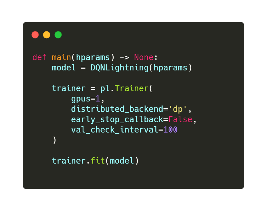
The last step is to call trainer.fit() on our model and watch it train. Below you can see the full Lightning code
After ~1200 steps you should see the agents total reward hitting the max score of 200. In order to see the reward metrics being plotted spin up tensorboards.
tensorboard --logdir lightning_logs

On the left you can see the reward for each step. Due to the nature of the environment this will always be 1, as the agent gets +1 for every step that the pole has not fallen (that’s all of the them). On the right we can see the total rewards for each episode. The agent quickly reaches the max reward and then fluctuates between great episodes and not so great.
You have now seen how easy and practical it is to utilize the power of PyTorch Lightning in your Reinforcement Learning projects.
This a very simple example just to illustrate the use of Lightning in RL, so there is a lot of room for improvement here. If you want to take this code as a template and try and implement your own agent, here are some things I would try.
I hope this article was helpful and will help kick start your own projects with Lightning. Happy coding!
The Ultimate Pytorch Research Framework